Written by: Ed Orlando, Data Scientist
Project Description
Anomaly detection can be valuable in many ways. For example, anomalies can be used to detect fraud, better understand system health monitoring, or help data engineers identify spikes in website traffic. It can also be used to remove extreme outliers from datasets before modeling.
In this project, webpage traffic outliers were identified that utilized data from the calendar year 2016. The project focused on popular United States sports, entertainment, and political events and people.
This project applied the anomalize package to assist in identifying outliers.
Interactive Tableau Public Viz
A Tableau interactive viz was created that used the final output produced in this project. The interactive viz can be viewed by clicking the link below.
Load Libraries
To get started, install/load the libraries listed below.
# 1.0 LIBRARIES ----
library(vroom)
library(tidyverse)
library(tidyquant)
library(lubridate)
library(rsample)
library(anomalize)
library(fuzzyjoin)
library(readxl)
Load Data
The original raw web data file included in the project can be downloaded here. The raw data was modified in a prior project I have offline since the original raw data file was very large (271 MB). I also created a couple lookup tables that create valuable features later in the pipeline.
To follow along, click here to download the sample files.
# 2.0 LOAD DATA ----
websites_sample_tbl <- vroom::vroom("Data_Sources/2020_06_15_Anomalize/websites_sample_tbl.csv", delim = ",")
page_summary_lkp_tbl <- read_xlsx("Data_Sources/2020_06_15_Anomalize/Topics_Dates_LKP.xlsx", sheet = "Sheet1")
topics_dates_lkp_tbl <- read_xlsx("Data_Sources/2020_06_15_Anomalize/Topics_Dates_LKP.xlsx", sheet = "Sheet2")
Subsets of the three (3) tibbles are listed below. The tibbles include information related to website traffic visits, the topic summary, details about the outliers, and the sources and links to the details.
head(websites_sample_tbl)
## # A tibble: 6 x 4
##    ...1 date       visits Page_Summary
##   <dbl> <date>      <dbl> <chr>
## 1     1 2015-10-01    683 1999_
## 2     2 2015-10-02    836 1999_
## 3     3 2015-10-03    742 1999_
## 4     4 2015-10-04    934 1999_
## 5     5 2015-10-05    778 1999_
## 6     6 2015-10-06    824 1999_
head(page_summary_lkp_tbl)
## # A tibble: 6 x 3
## Category Page_Summary Page_Summary_Formatted
## <chr> <chr> <chr>
## 1 Music & Entertainment The_Force_Awakens The Force Awakens
## 2 Music & Entertainment Leonardo_DiCaprio Leonardo DiCaprio
## 3 Music & Entertainment Matt_Damon Matt Damon
## 4 Music & Entertainment Brie_Larson Brie Larson
## 5 Music & Entertainment Room_ Room
## 6 Music & Entertainment Joy_ Joyhead(topics_dates_lkp_tbl)
## # A tibble: 6 x 4
## Page_Summary date Description Source
## <chr> <dttm> <chr> <chr>
## 1 1999_ 2016-04-21 00:00:00 On Apr 21, 2016, music le~ https://en.wikipe~
## 2 1999_ 2016-04-22 00:00:00 On Apr 21, 2016, music le~ https://en.wikipe~
## 3 1999_ 2016-04-23 00:00:00 On Apr 21, 2016, music le~ https://en.wikipe~
## 4 1999_ 2016-04-24 00:00:00 On Apr 21, 2016, music le~ https://en.wikipe~
## 5 1999_ 2016-04-25 00:00:00 On Apr 21, 2016, music le~ https://en.wikipe~
## 6 1999_ 2016-04-26 00:00:00 On Apr 21, 2016, music le~ https://en.wikipe~
Finding Anomalies
A few handy functions in the anomalize package were included in the analysis. The official descriptions included in the site above are listed below.
- time_decompose(): Separates the time series into seasonal, trend, and remainder components
- anomalize(): Applies anomaly detection methods to the remainder component.
- recomposed_l1 & recomposed_l2: added to calculate the limits that separate the “normal” data from the anomalies.
## ANOMALY DETECTION -----
websites_anomalies_tbl <- websites_sample_tbl %>%
    group_by(Page_Summary) %>%
    filter(is.na(date) == FALSE) %>%
    time_decompose(visits, method = "stl") %>%
    anomalize(remainder, method = "iqr", alpha = 0.014) %>%
    mutate(recomposed_l1 = season + trend + remainder_l1) %>%
    mutate(recomposed_l2 = season + trend + remainder_l2)
websites_anomalies_tbl %>% glimpse()
## Rows: 16,488
## Columns: 11
## Groups: Page_Summary [36]
## $ Page_Summary <chr> "1999_", "1999_", "1999_", "1999_", "1999_", "1999_",...
## $ date <date> 2015-10-01, 2015-10-02, 2015-10-03, 2015-10-04, 2015...
## $ observed <dbl> 683, 836, 742, 934, 778, 824, 892, 803, 884, 901, 923...
## $ season <dbl> -11.146825, 4.998995, 28.794452, 41.643661, -11.54451...
## $ trend <dbl> 816.7495, 815.6226, 814.4956, 813.3686, 812.2417, 811...
## $ remainder <dbl> -122.6027225, 15.3784293, -101.2900551, 78.9877085, -...
## $ remainder_l1 <dbl> -1940.961, -1940.961, -1940.961, -1940.961, -1940.961...
## $ remainder_l2 <dbl> 1979.766, 1979.766, 1979.766, 1979.766, 1979.766, 197...
## $ anomaly <chr> "No", "No", "No", "No", "No", "No", "No", "No", "No",...
## $ recomposed_l1 <dbl> -1135.359, -1120.340, -1097.671, -1085.949, -1140.264...
## $ recomposed_l2 <dbl> 2785.368, 2800.387, 2823.056, 2834.778, 2780.463, 276...Finally, an example of the anomalies viewed in R is listed below. The anomalize package includes a plot_anomalies() function that easily identifies the outliers.
In 2016, the Chicago Cubs were in the playoffs and eventually won the World Series. The popularity of that event is obviously apparent in the visual below.
websites_anomalies_tbl %>%
  filter(Page_Summary == "Chicago_Cubs") %>%
  filter(date >= as.Date("2016-01-01")) %>%
  plot_anomalies(ncol = 2, time_recomposed = TRUE)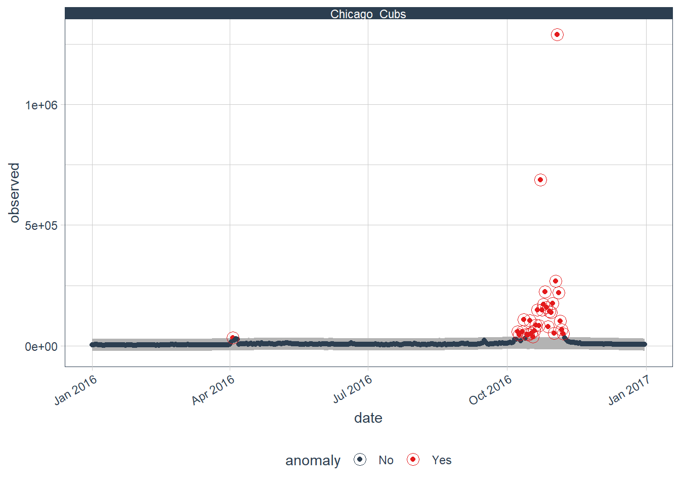
To view the fully interactive Tableau Public viz with all 2016 popular topics listed, please click here.
Final Tidy Tibble With Proper Titles & Descriptions
Finally, we can add the web page Category, Proper Title, Description of Outlier Event, and the Source. This tibble is what is exported and loaded into the Tableau Public viz.
websites_tidy_tbl <- websites_anomalies_tbl %>%
    left_join(page_summary_lkp_tbl) %>%
    left_join(topics_dates_lkp_tbl)
websites_tidy_tbl %>% glimpse()
## Rows: 16,490
## Columns: 15
## Groups: Page_Summary [36]
## $ Page_Summary <chr> "1999_", "1999_", "1999_", "1999_", "1999_",...
## $ date <dttm> 2015-10-01, 2015-10-02, 2015-10-03, 2015-10...
## $ observed <dbl> 683, 836, 742, 934, 778, 824, 892, 803, 884,...
## $ season <dbl> -11.146825, 4.998995, 28.794452, 41.643661, ...
## $ trend <dbl> 816.7495, 815.6226, 814.4956, 813.3686, 812....
## $ remainder <dbl> -122.6027225, 15.3784293, -101.2900551, 78.9...
## $ remainder_l1 <dbl> -1940.961, -1940.961, -1940.961, -1940.961, ...
## $ remainder_l2 <dbl> 1979.766, 1979.766, 1979.766, 1979.766, 1979...
## $ anomaly <chr> "No", "No", "No", "No", "No", "No", "No", "N...
## $ recomposed_l1 <dbl> -1135.359, -1120.340, -1097.671, -1085.949, ...
## $ recomposed_l2 <dbl> 2785.368, 2800.387, 2823.056, 2834.778, 2780...
## $ Category <chr> "Music & Entertainment", "Music & Entertainm...
## $ Page_Summary_Formatted <chr> "Prince", "Prince", "Prince", "Prince", "Pri...
## $ Description <chr> NA, NA, NA, NA, NA, NA, NA, NA, NA, NA, NA, ...
## $ Source <chr> NA, NA, NA, NA, NA, NA, NA, NA, NA, NA, NA, ...
For questions related to this analysis, please message me on LinkedIn.
For access to more of my articles, please check out my blog.